If you're reading about complexity, you may come across some terminology like Big O notation and asymptotic complexity, where an algorithm that takes about steps is referred to as .
Big O notation is a precise way to talk about complexity, and is referred to as "asymptotic complexity", which simply means how an algorithm performs for large values of .
The "asymptotic" part means "as gets really large" – when this happens, you are less worried about small details of the running time.
If an algorithm is going to take seven days to complete, it's not that interesting to find out that it's actually 7 days, 1 hour, 3 minutes and 4.33 seconds, and it's not worth wasting time to work it out precisely.
With asymptotic complexity we will make rough estimates of the number of operations that an algorithm will go through.
There's no need to get too hung up on precision since computer scientists are comfortable with a simple characterisation that gives a ballpark indication of speed.
For example, consider using selection sort to put a list of values into increasing order (this is explained in the chapter on algorithms).
Suppose someone tells you that it takes 30 seconds to sort a thousand items.
Does that sound like a good algorithm?
For a start, you'd probably want to know what sort of computer it was running on – if it's a supercomputer then that's not so good; but if it's a tiny low-power device like a smartphone then maybe it's ok.
Also, a single data point doesn't tell you how well the system will work with larger problems.
If the selection sort algorithm above was given 10 thousand items to sort, it would probably take about 50 minutes (3000 seconds) – that's 100 times as long to process 10 times as much input.
These data points for a particular computer are useful for getting an idea of the performance (that is, complexity) of the algorithm, but they don't give a clear picture.
It turns out that we can work out how many steps the selection sort algorithm will take for items: it will require about operations, or in expanded form, operations.
This formula applies regardless of the kind of computer it's running on, and while it doesn't tell us the time that will be taken, it can help us to work out if it's going to be reasonable.
From the above formula we can see why it gets bad for large values of : the number of steps taken increases with the square of the size of the input.
Putting in a value of 1,000 for tells us that it will use 1,000,000/2 - 1,000/2 steps, which is 499,500 steps.
Notice that the second part (1000/2) makes little difference to the calculation.
If we just use the part of the formula, the estimate will be out by 0.1%, and quite frankly, the user won't notice if it takes 20 seconds or 19.98 seconds.
That's the point of asymptotic complexity – we only need to focus on the most significant part of the formula, which contains .
Also, since measuring the number of steps is independent of the computer it will run on, it doesn't really matter if it's described as or .
The amount of time it takes will be proportional to both of these formulas, so we might as well simplify it to .
This is only a rough characterisation of the selection sort algorithm, but it tells us a lot about it, and this level of accuracy is widely used to quickly but fairly accurately characterise the complexity of an algorithm.
In this chapter we'll be using similar crude characterisations because they are usually enough to know if an algorithm is likely to finish in a reasonable time or not.
The complexity calculations for a simple algorithm can be measured in steps in the algorithm.
A more formal way of writing this is using "big-o" notation, such as , which is a quick and simple way to characterise an algorithm based on the number of values it has to process.
Basically it's a rough guide on to how quickly the complexity increases based on the size of the problem.
The size of the problem is most commonly written as the variable .
For example, searching a list of values for a given key, or sorting a list of values in ascending order.
As an example, the average case of sequential search takes about twice as long if it has twice as much data.
The time taken is proportional to , and this is simplified to in "big-o" notation.
Even if an algorithm takes steps, we write it as , since the time taken will be proportional to .
The big-o notation is called "asymptotic" complexity because "asymptote" means what happens as gets very large.
We don't worry much about values of , since in computer science we're usually dealing with thousands, millions, or billions of items of data.
If an algorithm takes step, and is a million, then it's accurate enough to say it takes about a million steps, the details aren't a big deal, and so it is characterised as , and not .
: this means the algorithm always takes the same amount of time regardless of the size of the input (the time taken is proportional to the number 1).
The best case of a sequential search is , which is when the first item checked happens to be the key being searched for.
This best case doesn’t depend on (the amount of items being searched).
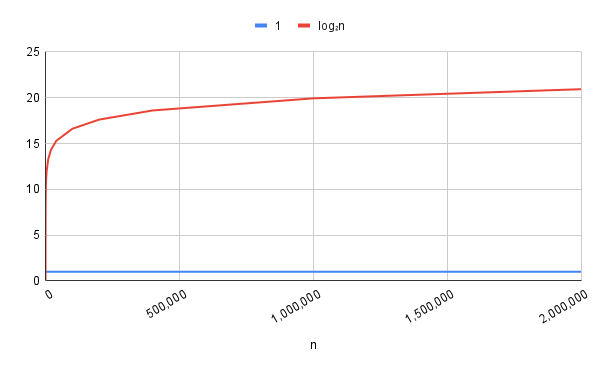
: This is proportional to the logarithm of .
Logarithms grow very slowly as increases, as shown in the graph below.
Binary search in the average and worst case is , because it divides the size of the problem in half at each step.
Logarithmic complexity is considered to be extremely good, since even huge values of require very few steps (for example, the graph below shows how a binary search of a million items only needs about 20 steps, and for 2 million items, only 21 steps).
What is a logarithm?
Curiosity
The logarithm function is a very important concept when you’re studying algorithms.
It can be confusing because algorithms and logarithms look like almost the same words, but they have very different meanings.
Here’s an example of the simple mathematics that is wrapped up in a logarithm: imagine that you fold a piece of paper in half, so that it is now 2 sheets thick.
Then you fold it again, so it is 4 sheets thick.
How many times to you need to fold it until it is 32 sheets thick?
The answer is that you need to fold it 5 times; using mathematical terminology, the logarithm of 32 is 5.
In general, the number of folds that you need to make is the logarithm of the thickness of the folded paper.
To get the paper 1024 sheets thick, you need to fold it 10 times, and the logarithm of 1024 is 10.
Following this reasoning, the logarithm of 1,048,576 is 20 (yup, just 20 folds will make the paper over a million pages thick, if you could somehow fold it 20 times.)
The mathematical shorthand for logarithm is log. For example,
Strictly speaking, a logarithm also has a “base”; in the example the base is 2, because we are doubling the thickness with each fold, so to be precise, we would use the subscript 2 to indicate this:
Another way of thinking of a logarithm is that it’s the number of times you can divide something in half until you get one item (which is really just the paper folding in reverse).
So if you start with the number 32, then halve it to 16, then again to 8, 4, 2 and 1, you have done 5 halvings; is 5.
One place where we’ve already seen a logarithm at work is in binary search.
Because binary search halves the number of items to search at each step, it takes at most to search items; for example, it takes at most 20 steps to search 1,048,576 items.
From these examples, you can see that the logarithm function grows very slowly; even a billion items only takes 30 steps.
So when we see that the complexity of an algorithm is logarithmic, it’s great news.
Even a vast amount of input data will take a fraction of a second to process.
An easy way to calculate is to use a spreadsheet; usually you can use a formula like this (the 2 means that it is base 2):
=log(A1,2)
Pocket calculators don’t normally have a button, but you will probably find . You can calculate by working out .
In case you’re wondering, logarithms are the inverse of exponential functions. Exponential functions get huge really quickly; logarithms are the opposite. The relationship is that if , then .
The above graph also shows the shape of the function for the value 1 (in blue).
It’s just a horizontal line!
A typical algorithm might actually take a few operations when it runs, but as long as it’s a constant number, then it’s proportional to the value 1, and we write it as , which just means a constant value.
Although we’ve drawn the graphs here, it’s really informative to draw your own ones, to get a feel just how different these functions are.
And bear in mind that this is often the kind of difference in performance between two algorithms that solve exactly the same problem!
: this means the time taken is roughly proportional to the amount of input.
Sequential search (average and worst case) are , because searching twice as much data will take about twice as long.
The best case of insertion sort in , which happens when it is given a list that is nearly in sorted order; this is actually useful in combination with faster algorithms such as quicksort.
: this is only slightly worse than , since the “log n” factor is relatively small.
The best sorting algorithms take O(n log n) time on average, and in the best case (including mergesort and quicksort).
Mergesort is also in the worst case, but quicksort can be in the worst case.
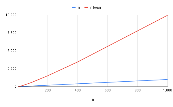
The following graph plots the value (which is just a straight line), and , which looks almost straight, but bends up very slightly since increases very slightly as increases.
But isn’t much worse than as far as asymptotic complexity goes.
In the graph below it’s about 10 times worse on the right hand side, but remember that we’re not too worried about constant factors, just the rate of growth.
: The time taken increased roughly in proportion to the square of the amount of data.
For example, twice as much data would take 4 times as long; 10 times as much data would take 100 times as long.
Common algorithms that use this amount of time are selection sort (best, worst and average cases), insertion sort (average and worst case), bubblesort (average and worst case).
These algorithms aren’t usually used in practice because the speed is bad for large amounts of data (except insertion sort has some specialist use).
is sometimes referred to as “quadratic”, since it’s based on a quadratic equation.
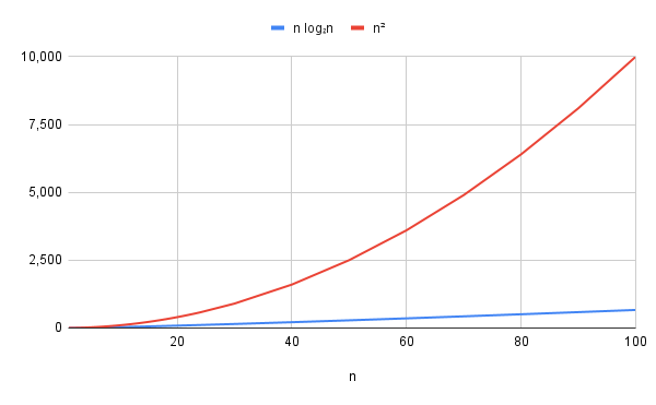
The following graph plots , which is the parabola shape that a quadratic function produces.
The key thing is that this function increases faster and faster as increases, so it’s really not very good. Notice that the x axis only goes up to 100 here, so an algorithm isn’t likely to be very good for even moderately large numbers.
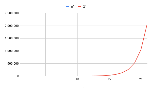
: This grows incredibly fast - it is called exponential growth because is in the exponent.
For example, for = 100 (just 100 items to process), try calculating and see how much more time an exponential-time algorithm will take compared with a quadratic-time algorithm using steps.
Algorithms that are are usually trying out every possible solution to find which is best.
Examples include generating all subsets of a set of items; and trying all combinations of vertices in vertex cover.
The following chart compares with - you can hardly see the blue line (it looks like it’s stuck at the bottom) - the exponential line just heads for the roof impossibly fast.
: This is factorial time, and usually comes up when trying every order that a set of items can be placed in.
A brute-force solution to the Travelling Salesperson problem does this; after the starting point, there’s a choice of places to visit first, then to visit second, and so on.
This works out at orderings for visiting all the locations.
This value grows incredible fast as increases.